Introduction and goals
Before starting this lesson, I often warn students that “this is the most boring lesson, but it is also the most important, by far”. For me, one of the largest hurdles for me in learning LiDAR shear volume of data, which I hadn’t yet become accostomed. Often, it was more difficult learning workarounds for cumbersome datasets than understanding the algorithm I was trying to employ.
As you work with larger datasets, you will need to learn how to speed up the analyses. In the previous modules, we worked with a 1 km2 area of forest and created digital elevation models, canopy height models, and mapped individual trees and their crowns.
Some of these steps took a few seconds. For the most part, they can be quick on a standard desktop computer. However, as you begin working with larger datasets, it will be useful to learn ways to speed up the analysis. We can do this by reducing the data in some way. This could mean focusing on a smaller area of interest. Or we can load a lower resolution version of the data when high resolution data is not needed.
In the remaining modules, you will learn techniques for speeding up your LiDAR analyses. By the end of this module, you will learn techniques for creating reduced datasets. You will be able to:
- Create a spatial index to speed up loading reduced datasets
- Subset a LiDAR scene to focus on a smaller area of interest
- Create a lower density point cloud when lower resolution data is acceptable
Create a spatial index (*.lax)
Loading data from the hard drive into memory can be a slow process. If you do not need the full dataset, it can be useful to load a reduced version. For example, you may only need one small subsection, or you may be able to use a reduced resolution. But there is a problem. How can you filter out datasets without loading the entire file in the first place?
Creating an index can solve this problem. Indexing your LiDAR data creates a small file (*.lax). The index file contains an overview of the structure of the LiDAR data contained in the main LiDAR file (.las or .laz). The index files contain a map of information on where data is located, so that the lidR package can load only specified portions of the file into memory.
For example, you may only want to load data that is 20 m around a specified coordinate. Or you may be interested in an area defined by a specific bounding box. Or you may want to thin the points, and only load one point every 10 cm.
Creating an index is simple with the writelax function from the rlas package. We have also created the check_for_lax function in the landecoutils package which allows you to create index files for multiple files which we will do in the next module (Module 6: Speed up your analyses: Parallel processing with LAScatalog). Important Note: The landeocutils package uses a now defunct dependency, so you have to also install TreeLS and spanner packages. We will cover this in the next module.
# You should already have this package installed since the `lidR` package depends on it.
library(rlas)

#indicate the path to the filename of the .las/.laz that you want to index.
writelax('NEON_D03_JERC_DP1_740000_3459000_classified_point_cloud.laz' )
You will notice that a new file has been created in the same folder that the .laz file was located. It will share the same base name, but end with a .lax extension. The lidR package requires the basename of an index file to match its the main .laz or .las file it corresponds to.
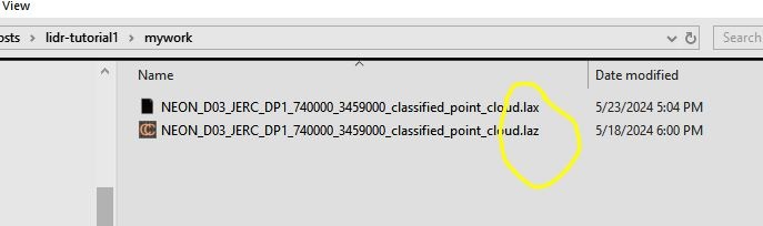
*.laz) and its corresponding index file (*.lax)Load a subset of a LiDAR scene
Now that you have created an index, you can quickly load smaller subsets of the data. To do this, you add a filter = argument to the readLAS function. for example -keep_xy xmin ymin xmax ymax will keep all the LiDAR returns between the bounding box specified by the appropriate coordinates. If you want a circular area, you can specify it with the coordinate of the circle center and the radius (-keep_circle X Y R). Try these functions below and note the time differences from loading the full las file.
library(lidR)
# Subset within the bounding box specified by the UTM16 coordinates 740400 3459500 740500 3459600
las = readLAS('NEON_D03_JERC_DP1_740000_3459000_classified_point_cloud.laz',
        filter = '-keep_xy 740400 3459500 740500 3459600') #xmin ymin xmax ymax
las = filter_poi(las, Z < 300) #don't forget to drop noise
view(las) # You may not need the `lidRViewer` backend since this is a smaller point cloud!

# Subset a 30 m circular area around the coordinate 740400 3459500
las = readLAS('NEON_D03_JERC_DP1_740000_3459000_classified_point_cloud.laz',
        filter = '-keep_circle 740400 3459500 30') #xcenter ycenter radius
las = filter_poi(las, Z < 300)
view(las)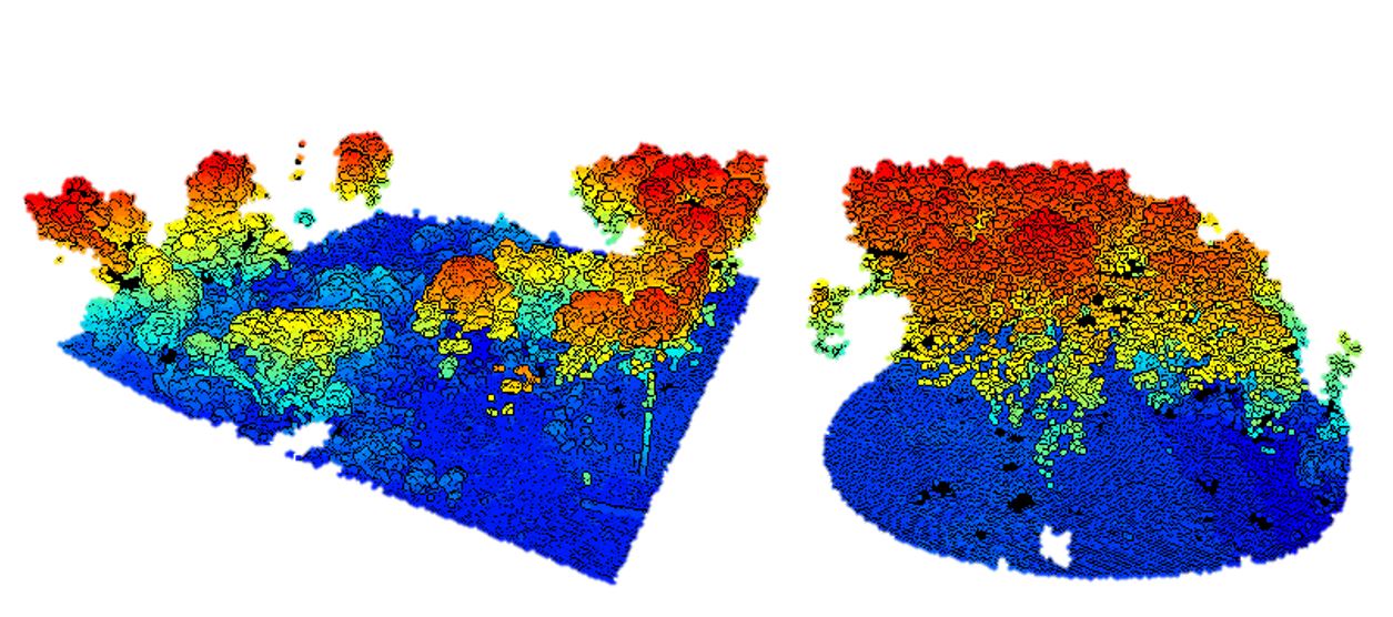
filter argument from the readLAS functionSometimes it may be useful to thin the data. You can do this in a few ways. You could load only a random fraction, say 10%, of an entire datase using the -keep_random_fraction tag. LiDAR scans do not always result in an equal point density across a scene. If it is important for all areas of the scene to have an equal point density, you may want to use the -thin_with_grid option. One especially useful option is the -thin_with_voxel tag which loads only 1 random return in each voxel volume. We use this frequently with terrestrial LiDAR data.
You can also combine multiple filters. See the last example, where we -drop_z_above to simultaneously filter out the noise we learned about earlier.
# Thin the LiDAR scene randomly to 10% of its original density
las = readLAS('NEON_D03_JERC_DP1_740000_3459000_classified_point_cloud.laz',
            filter = '-keep_random_fraction 0.1')
las = filter_poi(las, Z < 300 & Z > 30)
view(las)

# Load one point every 2 m. Useful for a coarse DEM or CHM
las = readLAS('NEON_D03_JERC_DP1_740000_3459000_classified_point_cloud.laz',
            filter = '-thin_with_grid 2')
las = filter_poi(las, Z < 300 & Z > 30)
view(las)

# Load one point in every 0.5 x 0.5 x 0.5 m voxel.
las = readLAS('NEON_D03_JERC_DP1_740000_3459000_classified_point_cloud.laz',
            filter = '-thin_with_voxel 0.5 -drop_z_above 90 -drop_z_below 20')
#las = filter_poi(las, Z < 300) #noise filter not needed since drop z took care of it.
view(las)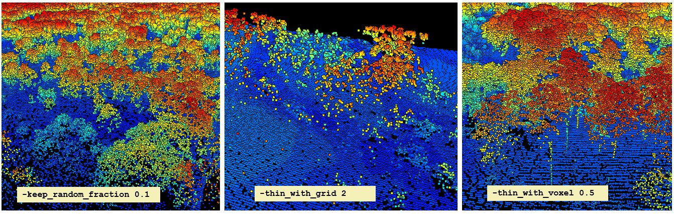
We have looked at six different filters here, but you can also filter on attributes such as RGB values, intensity, scan angle, and more. You can use the command readLAS(filter = "-help") anytime to see a complete list. Try out some others!
readLAS(filter = "-help")Filter points based on their coordinates.
-keep_tile 631000 4834000 1000 (ll_x ll_y size)
-keep_circle 630250.00 4834750.00 100 (x y radius)
-keep_xy 630000 4834000 631000 4836000 (min_x min_y max_x max_y)
-drop_xy 630000 4834000 631000 4836000 (min_x min_y max_x max_y)
-keep_x 631500.50 631501.00 (min_x max_x)
-drop_x 631500.50 631501.00 (min_x max_x)
-drop_x_below 630000.50 (min_x)
-drop_x_above 630500.50 (max_x)
-keep_y 4834500.25 4834550.25 (min_y max_y)
-drop_y 4834500.25 4834550.25 (min_y max_y)
-drop_y_below 4834500.25 (min_y)
-drop_y_above 4836000.75 (max_y)
-keep_z 11.125 130.725 (min_z max_z)
-drop_z 11.125 130.725 (min_z max_z)
-drop_z_below 11.125 (min_z)
-drop_z_above 130.725 (max_z)
-keep_xyz 620000 4830000 100 621000 4831000 200 (min_x min_y min_z max_x max_y max_z)
-drop_xyz 620000 4830000 100 621000 4831000 200 (min_x min_y min_z max_x max_y max_z)
Filter points based on their return numbering.
-keep_first -first_only -drop_first
-keep_last -last_only -drop_last
-keep_second_last -drop_second_last
-keep_first_of_many -keep_last_of_many
-drop_first_of_many -drop_last_of_many
-keep_middle -drop_middle
-keep_return 1 2 3
-drop_return 3 4
-keep_single -drop_single
-keep_double -drop_double
-keep_triple -drop_triple
-keep_quadruple -drop_quadruple
-keep_number_of_returns 5
-drop_number_of_returns 0
Filter points based on the scanline flags.
-drop_scan_direction 0
-keep_scan_direction_change
-keep_edge_of_flight_line
Filter points based on their intensity.
-keep_intensity 20 380
-drop_intensity_below 20
-drop_intensity_above 380
-drop_intensity_between 4000 5000
Filter points based on classifications or flags.
-keep_class 1 3 7
-drop_class 4 2
-keep_extended_class 43
-drop_extended_class 129 135
-drop_synthetic -keep_synthetic
-drop_keypoint -keep_keypoint
-drop_withheld -keep_withheld
-drop_overlap -keep_overlap
Filter points based on their user data.
-keep_user_data 1
-drop_user_data 255
-keep_user_data_below 50
-keep_user_data_above 150
-keep_user_data_between 10 20
-drop_user_data_below 1
-drop_user_data_above 100
-drop_user_data_between 10 40
Filter points based on their point source ID.
-keep_point_source 3
-keep_point_source_between 2 6
-drop_point_source 27
-drop_point_source_below 6
-drop_point_source_above 15
-drop_point_source_between 17 21
Filter points based on their scan angle.
-keep_scan_angle -15 15
-drop_abs_scan_angle_above 15
-drop_abs_scan_angle_below 1
-drop_scan_angle_below -15
-drop_scan_angle_above 15
-drop_scan_angle_between -25 -23
Filter points based on their gps time.
-keep_gps_time 11.125 130.725
-drop_gps_time_below 11.125
-drop_gps_time_above 130.725
-drop_gps_time_between 22.0 48.0
Filter points based on their RGB/CIR/NIR channels.
-keep_RGB_red 1 1
-drop_RGB_red 5000 20000
-keep_RGB_green 30 100
-drop_RGB_green 2000 10000
-keep_RGB_blue 0 0
-keep_RGB_nir 64 127
-keep_RGB_greenness 200 65535
-keep_NDVI 0.2 0.7 -keep_NDVI_from_CIR -0.1 0.5
-keep_NDVI_intensity_is_NIR 0.4 0.8 -keep_NDVI_green_is_NIR -0.2 0.2
Filter points based on their wavepacket.
-keep_wavepacket 0
-drop_wavepacket 3
Filter points based on extra attributes.
-keep_attribute_above 0 5.0
-drop_attribute_below 1 1.5
Filter points with simple thinning.
-keep_every_nth 2 -drop_every_nth 3
-keep_random_fraction 0.1
-keep_random_fraction 0.1 4711
-thin_with_grid 1.0
-thin_with_voxel 0.1
-thin_pulses_with_time 0.0001
-thin_points_with_time 0.000001
Boolean combination of filters.
-filter_andNext Steps
Now you have a few tools that will help you begin to work with larger datasets. Reducing the extent or resolution of data can help speed up some analyses immensely. But high detail is needed for some others.
In the next module you will begin to learn how to use tools in the lidR package to harness the power of parallel processing. This will increase the speed and extent to which you can analyze LiDAR data.
In the next module you will:
- Acquire and load a large LiDAR dataset
- Set
chunkoptions withLAScatalog - Consider edge effects
- Get an introduction to
catalog_applyand parallel processing
Continue learning
- Module 1: Acquiring, loading, and viewing LiDAR data
- Module 2: Creating raster products from point clouds
- Module 3: Mapping trees from aerial LiDAR data
- Module 4: Putting it all together: Asking ecological questions
- Module 5: Speeding up your analyses: Reduced datasets
- Module 6: Speed up your analyses: Parallel processing with LAScatalog
- Module 7: Putting it all together (large-scale raster products)