Introduction and goals
In the last module, we covered how to work with LiDAR data including how to acquire, load, de-noise, and view the data in R. In this module, we will advance to basic analysis. By the end of this module, you should be able to:
- generate a digital elevation model from LiDAR data
- generate a canopy height model from LiDAR data
Making a digital elevation model is often the first step in many LiDAR analyses. Even when elevation is not strictly of interest, it is useful to know where the ground is located so that the height of objects (e.g., buildings or trees) can be measured relative to the ground.
Note: Many commercial LiDAR products often come with a digital elevation model, or already have points classified as ground. That includes the NEON dataset we use here. Nevertheless, it can be useful to understand the principles and steps involved so that you can make your own elevation models as needed, or recreate them at other scales.
Downloading R packages
You will need several packages to get started. In the previous module (Module 1: Acquiring, loading, and viewing LiDAR data), you should have installed lidR, lidRviewer, and devtools. You will also need one new package:
terra:terrais anRpackage that is the new standard for working with raster data. It recently replaced the deprecatedrasterpackage. I find it to be faster, and it is more compatible with thelidRandsfpackages and other spatial analysis packages.
# install CRAN packages if you haven't already
install.packages('terra')

library(lidR)
library(lidRviewer)
library(terra)
Loading and de-noising LiDAR data
- Download this sample LiDAR dataset used in the previous module. Load and de-noise the LAS object to prepare for analysis. If you need a refresher for how to load and de-noise, check the previous module (Module 1: Acquiring, loading, and viewing LiDAR data).
# Load example dataset above, or path to your data.
las = readLAS('NEON_D03_JERC_DP1_740000_3459000_classified_point_cloud.laz')

# or if you downloaded the reduced dataset instead
# las = readLAS('NEON_D03_JERC_DP1_740000_3459000_classified_point_cloud-reduced.laz')

# Classify all isolated returns. Takes a few seconds
las = classify_noise(las, ivf(res = 3, n = 10))

# Filter out the noise
las = filter_poi(las, Classification != LASNOISE)

# The highest point value has a Z of 972.81. Keep only points below it.
max(las$Z)
las = filter_poi(las, Z < 970)
view(las)
# Press the z-key to view it colored by height
Making a digital elevation model (DEM)
The first step in generating a digital elevation model is to decide which points in the LiDAR scene represent the GROUND. In principle, you can designate returns with the lowest elevation (Z) in every, say 1 m2 area to represent ground. However, this can be messy depending on the presence of vegetation, shadows, reflections, and noise.
Instead, it is standard to use a cloth simulation filter which is available through the LiDAR function csf(). With the csf function, the LiDAR point cloud is inverted, and a simulation of a “rigid cloth” is draped over the inverted point cloud. The simulated cloth surface is then used to determine which points are associated with the ground.

Example of cloth simulation which can be adapted to identify ground pounts by inverting lidar scenes. Source: Wikimedia Commons.
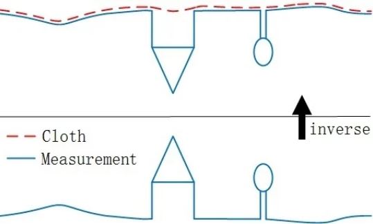
Diagram illustrating cloth simulation filter. From Zhang et al. (2016).
Once points are classified, you know which points are associated with the ground, but because points are not continuous on the ground, you still need to interpolate between them to get an elevation map. For this, you can use a Delaunay triangulation which interpolates a continuous surface as a triangulation between the points classified as ground. You can implement the tringulation using the rasterize_terrain() function in the lidR package with the tin() algorithm selected.
las = classify_ground(las, algorithm = csf()) #see `?csf for more algorithm options
# This may take a little while. We'll learn how to 'thin' point clouds later
# You may get a warning that the points were already classified.
# That's because NEON data comes pre-classified. But that's not always the case!

view(las)
#Press the c-key to view the classified points, that include ground points

dem = rasterize_terrain(las, res=1, algorithm=tin())

plot(dem)

# You can also make a slope or aspect map,
# Note these contain less noise when using coarser resolution dem. Try making one!
slope = terrain(dem, v='slope', unit='degrees')
asp = terrain(dem, v='aspect', unit='degrees')

par(mfrow=c(1,2)) # make a 1x2 panel plot window
plot(slope)
plot(asp)

writeRaster(dem, 'dem.tiff')
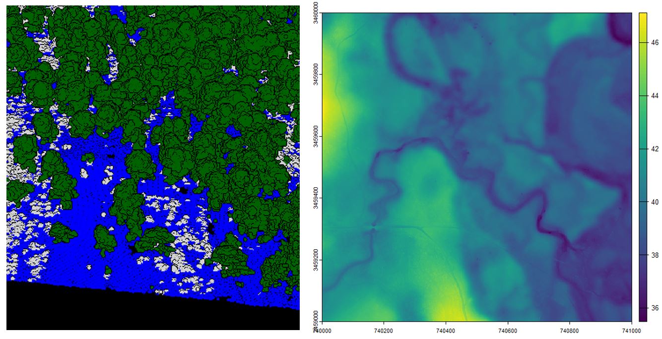
Left. Classified LiDAR returns, blue points represent returns classified as ground. Green and white points were previously classified as high- and low-vegetation. Right. Digital elevation model produced at a 1 m resolution
With the terra package, you can plot the raster data and reveal the rich landscape built by subtle changes in topography. This area reveals the subtle topographic changes (~10 m) in a southeastern floodplain forest and its associated uplands. You can also spot some faint dirt roads in yellow near the southwestern corner.
The terra package is also useful for working with terrain data. Check out the terrain function where you can use the dem you just created to make rasters for slope and aspect.
Finally, you can use the writeRaster function from terra to save the dem (or other derived rasters you made). Save these as a *.tiff and you will have a geo-Tiff which has a coordinate reference system and so can be opened in software like ArcGIS.
Making a canopy height model
In the last section, we analyzed the ground returns to make a raster of the terrain. It can also be useful to know the actual heights of objects (relative to the ground). The basic process is to identify the elevation of the trees (a so-called canopy surface model) and then subtract the terrain underneath to create a canopy height model. To accomplish this, we will use another function made for this purpose from the terra package called rasterize_canopy().
# First make a canopy surface model
csm = rasterize_canopy(las, algorithm = pitfree())

# Make a canopy height model by subtracting the csm from the dem
chm = csm - dem

par(mfrow = c(1,3), mar=c(1,1,3,2))
plot(dem, main='digital elevation model')
plot(csm, main='canopy surface model')
plot(chm, main='canopy height model')
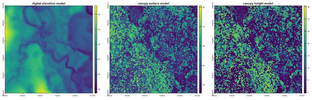
Raster products showing basic terrain and canopy heights from the lidR package
Other raster products
Understory density
You can use the rasterize_density tool in creative ways to calculate point density at different heights. For example, if you are interested in wildlife habitat, you may wish to know about the density of understory vegetation. Among wildlife species in open habitats, many seek dense vegetation near the surface for cover. Perhaps you wanted to know where the understory vegetation was most dense. You can look at the vegetation between, say, 0 and 1 m high, and calculate the density of points that are found there. This provides an index to some on-the-ground metric such as herbaceous biomass.
To do to this you can “normalize” the point cloud (flatten out the effects of terrain), remove all the ground points and points > 1 m, and then estimate their density relative to the density of all points in that column. Remember: that aerial LiDAR returns are not evenly distributed across the scene. Some areas get passed by the the laser several times, and others just once. So, we need to relativize the point density from the understory to the total point density in a pixel.
# Normalize the `LAS` object, by subtracting out height
las.norm = normalize_height(las, algorithm=tin())
# Keep only points that are not ground and that are <2 m above ground
understory_points = filter_poi(las.norm, Classification != LASGROUND & Z < 2)
# Count the point density at a 10 m resolution. This could be an index of understory vegetation density
total_density = rasterize_density(las, res=10)
# Count the point density for ALL points
understory_only = rasterize_density(understory_points, res=10)
# Calculate the fraction of understory points relative to the total.
percent_understory_pts = understory_only / total_densitypar(mfrow = c(1,3), mar=c(1,1,3,2))
plot(understory_only)
plot(total_density)plot(percent_understory_pts)
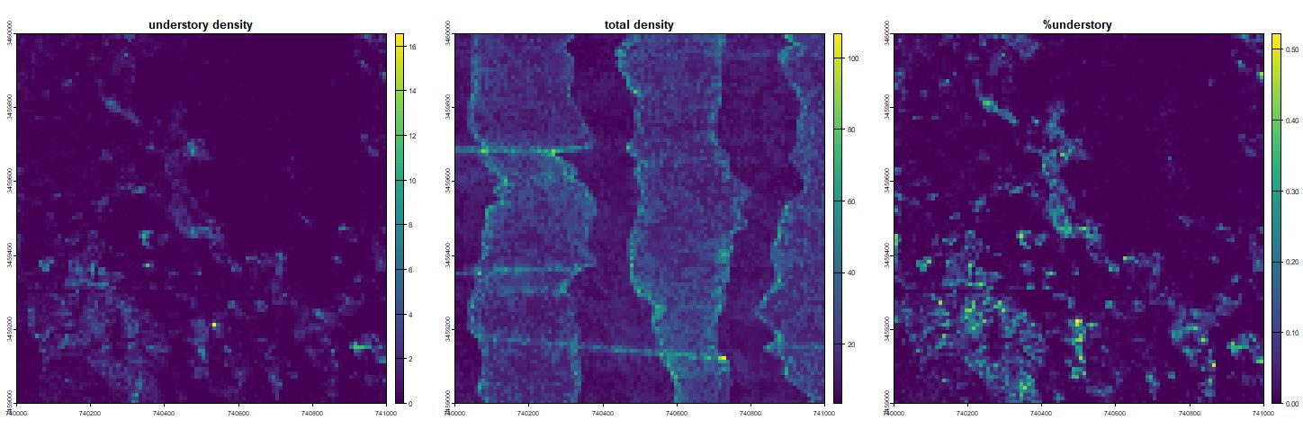
Left: Total number of understory returns in units of points per square meter. Center: Return density forms vertical stripes due to movement and overage of laser. Right: The propoportion of understory returns are high along streams and in the southwest corner. Perhaps the northeastern portion had been recently burned.
Write custom functions: Vegetation structural complexity
Ther rasterize_* functions all work in a similar way, including rasterize_heights, rasterize_density, and rasterize_terrain. They each summarize an attribute of a column of LiDAR data at some named resolution for every pixel. These are actually all special cases of the pixel_metrics function. More generally you can use the pixel_metrics function to write custom functions. Basically, for some given pixel resolution, you can retrieve the “column” of LiDAR points and summarize them for some attribute.
For example, structural complexity is another important aspect of wildlife habitat and a good indicator of tree regeneration. A structurally complex stand will have a mixture of short, medium, and tall vegetation. We could use the coefficient of variation at some scale to see if they are all present.
# first define a function that uses the an attirubte of the lidar data (e.g., Z value) to summarize some useful metric (in this case, we calculate a coefficiant of variation of heights (sd/mean))
my_complexity_function = function(Z) sd(Z)/mean(Z)
# and summarize it at some scale
complexity = pixel_metrics(las, my_complexity_function(Z), res = 10)par(mfrow = c(1,1), mar=c(1,1,3,2))
plot(complexity), main='complexity')
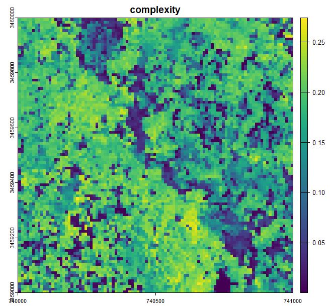
Structural complexity as measured by the coefficient of variation of return height
Next steps
Now you have started to learn to extract basic information from LiDAR point clouds such as topography and canopy heights. You have also started to make custom functions to process LiDAR data. As you’ll see, making customized functions is where LiDAR processing becomes really powerful!
In the next module you will learn to:
- Use a canopy height model to identify tree locations
- Individually segment trees and estimate tree size
- Turn a LiDAR point cloud into a stem map
Continue learning
- Module 1: Acquiring, loading, and viewing LiDAR data
- Module 2: Creating raster products from point clouds
- Module 3: Mapping trees from aerial LiDAR data
- Module 4: Putting it all together: Asking ecological questions
- Module 5: Speeding up your analyses: Reduced datasets
- Module 6: Speed up your analyses: Parallel processing with LAScatalog
- Module 7: Putting it all together (large-scale raster products)