Introduction and goals

Now you know how to aquire a large dataset, set options with LAScatalog, understand how to deal with edge effects, and the utility of parallel processing. Next, we will put all these steps to work and generate raster products (digital elevation model, etc.) for a very large area! After completing this module, you will be able to:

• Create a digital elevation model and stem map for a large area
• Divide a lidar dataset into many chunks to process seperately
• Deal with edge effects using the catalog_map function
• Utilize parallel processing to speed up analyses with the future package
• Combine all outputs into a single seamless product

Setup

We will start by retracing our steps. Load the lidR, landecoutils and terra packages. The landecoutils package must be loaded from GitHub. See the previous tutorial on how to do this (Module 6: Speed up your analyses: Parallel processing with LAScatalog). Create index files for your dataset if needed, and set chunk options. We will use a smaller area (500 m) so that our computer memory is not overwhelmed when we use parallel processing.

library(lidR)
library(landecoutils)
library(terra)
# Path to your lidar directory
dir = "C:/JERC/ClassifiedPointCloud/"

# my lab and JOnes Center staff can read directly from local copy of neon data
# dir = 'I:/neon/2023/lidar/ClassifiedPointCloud/'

# Make index files if needed.
# from landecoutils package, see previous module for instructions on installing 
# packages from GitHub
check_for_lax(dir) 

# Load the catalog object
ctg = readLAScatalog(dir) # may take a second.... 

# SEt some of the chunk options before, Making them smaller (500 m) but with 
# a small buffer, and thin to a 0.5 m voxel. 
opt_chunk_size(ctg) = 500
opt_chunk_buffer(ctg) = 10 
opt_chunk_alignment(ctg) = c(0,0)
opt_filter(ctg) = '-thin_with_voxel 0.5'

# Take a look at how these chunks line up with the boundaries
# of the source data.
plot(ctg, chunk_pattern = TRUE)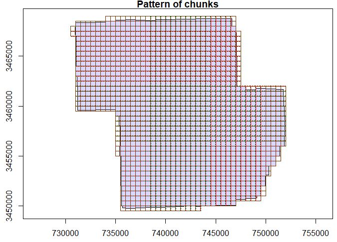

Create a function to run on each chunk

Before attempting to create a digital elevation model for an entire scene, it can be useful to first recall from previous modules (Module 2: Creating raster products from point clouds) how we created a DEM for a single tile or chunk. We read in the data using readLAS, and we classified noise (with classify_noise) and removed it (with filter_poi). We identified the ground points with classify_ground, and finally, we generated the dem with rasterize_terrain.

# load the LAS object from a a filename
las = readLAS('NEON_D03_JERC_DP1_740000_3459000_classified_point_cloud.laz')

# Create a digital elevation model (dem)
las = classify_noise(las, ivf(res = 3, n = 10))
las = filter_poi(las, Classification != LASNOISE)
las = classify_ground(las, algorithm = csf()) #see `?csf` for more options
dem = rasterize_terrain(las, res=1, algorithm=tin())

# Create a canopy surface model
csm = rasterize_canopy(las, algorithm = pitfree())

# Make a canopy height model by subtracting the csm from the dem
chm = csm - dem

# Combine all of these outputs into a 3-layered raster object
# The first half of each item in the list gives each layer a name in the rast object
combined_output = c(dem=dem, csm=csm, chm=chm)

# View and plot each one
par(mfrow = c(1,3), mar=c(1,1,3,2))
plot(combined_output$dem, main='digital elevation model')
plot(combined_output$csm, main='canopy surface model')
plot(combined_output$chm, main='canopy height model')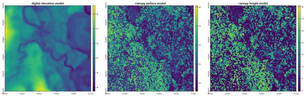

Raster products showing basic terrain and canopy heights from the lidR package

Now we will take these series of steps and convert them into a function. If you have not yet learned how to build custom functions, review this tutorial on creating functions in R. Note that in constructing this function, we merely repeat the same steps as above. We will need to create functions that can take as an argument a single las object and return whatever product we need such as a feature or raster object.

# Function takes a `las` object as an input and returns a raster (`rast` object)
# with three layers (dem, csm, chm)

myFunction = function(las) {
  las = classify_noise(las, ivf(res = 3, n = 10))
  las = filter_poi(las, Classification != LASNOISE)
  las = classify_ground(las, algorithm = csf()) #see `?csf` for more options
  dem = rasterize_terrain(las, res=1, algorithm=tin())
  csm = rasterize_canopy(las, algorithm = pitfree())
  chm = csm - dem
  combined_output = rast(c(dem=dem, csm=csm, chm=chm))
  return(combined_output)
}

Scaling up!

Now you have a (1) a lidar scene that is broken up into several chunks, and (2) a function that you can apply to each of those chunks to get an output. You are now ready to scale-up! You can use the catalog_map function from the lidR package which allows you to take two arguments: (1) a LAScatalog object containing information on your lidR scene (ctg in our example), and (2) a function to apply to each of the chunks in that scene (myFunction in our example).

Using the catalog_map function also has two other very handy features. It can manage edge effects and parallel processing which are important considerations as we scale up.

1. Edge effects: We specified a small buffer, opt_buffer = 10 above. That tells the catalog_map function to include an additional 10 m buffer each time it works on a chunk. But when the operation is complete, the function will trim that 10 m buffer off, so that each piece of output will fit back together seamlessly.
2. Parallel processing: By breaking the LiDAR scene into chunks, we can process each one independently. So, each core of your computer can work on a different chunk simultaneously! In order to use the parallel processing features, you will need an additional R package called future which lets you specify the number of cores to use at once. We will use 4 cores, but you may want to use more or fewer depending on your computer resources and chunk sizes.

install.packages('future')
library(future)

# Set the number of cores to use using the `plan` and `multisession` functions
plan(multisession, workers = 4)

# Let's say we are interested in a smaller aresa, we can also 
# clip `ctg` down to smaller area by adding `keep_xy` to our filter
opt_filter(ctg) = '-thin_with_voxel 0.5 -keep_xy 735000 3450000 740000 3455000'

# Now use the `catalog_map` function using your `ctg` and user-defined dem function
output = catalog_map(ctg, myFunction) #will take a while 

If you are using RStudio, you can watch the plot window as your chunks are processed in real time. Green squares indicate that a chunk is successfully completed and processed. Grey squares are those that have been checked, but lie outside of the extent we specified with opt_filter. Orange squares indicate that a chunk completed successfully but with a warning. Blue squares represent chunks that are currently processing. (Note that the plot seems to have a lag as there are 5 chunks indicated as processing, but we specified 4 workers.)

Diagram indicating processing progress of myFunction using 4 cores

As you use different processes, you may need to take care to watch your computer resources. Use Ctl + Alt + Del in windows and view your Task Manager when trying a new process. Pay careful attention to your CPU and RAM resources. If your process is using CPU or RAM exceeding 80-90%, then performance becomes sluggish. You may need to reduce the size of your chunks, or reduce the number cores you are using. Resource use scales differently depending on the alogrithms you are using. In some cases, doubling the chunk area will double resources (as in our example). But in other cases, increasing chunk area can increase computer resources exponentially (as in the case of some distance-based operations). Read about Big O Notation to learn more about why.

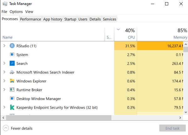
Check in on resource use as you test and implement new algorithms

View and save the outputs

The catalog_map function also manages merging all the outputs from individual chunks. Each output is a non-overlapping raster tile that is merged into a single raster. View the outputs, which cover a much larger area by plotting them. Last, you can save your outputs as a GEOTiff using the writeRaster command.

You can tell by the canopy height model that this portion of the scene is characterized by fragmented forests and agricultural fields. The circular areas with no canopy are circular agricultural fields with pivot irrigation. This area is located outside of the main longleaf pine conservation area that is the focus of this NEON site.

# View and plot each one
par(mfrow = c(1,3), mar=c(1,1,3,2))
plot(output)

# Save these outputs to use later. 
# Export the entire 3-layer raster
writeRaster(output, 'C:/User/Me/Desktop/myOutput.tiff')

# You can also export a specific layer as a GEOTiff.
# Let's output the DEM and the CHM to use in the next module.
writeRaster(output$chm, 'C:/User/Me/Desktop/myCHM.tiff')
writeRaster(output$dem, 'C:/User/Me/Desktop/myDEM.tiff')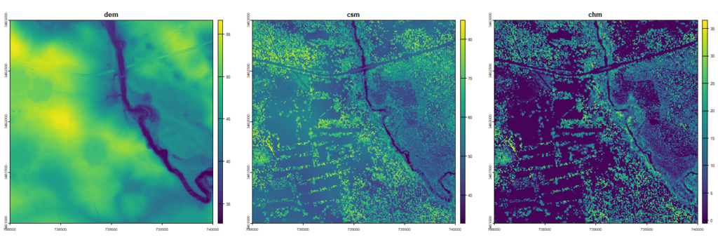

Raster output for 16 km² area showing a digital elevation model (dem), a canopy surface model (csm), and a canopy height model (chm)

Next steps

Now you have combined the previous steps and are able to work with very large datasets, deal with edge-effects, and harness the power of parallel processing. You created a digital elevation model and other elevation-based products.

The next step in proficiency with lidar will be to develop your own questions and algorithms! Get crackin!

Review modules

• Module 1: Acquiring, loading, and viewing LiDAR data
• Module 2: Creating raster products from point clouds
• Module 3: Mapping trees from aerial LiDAR data
• Module 4: Putting it all together: Asking ecological questions
• Module 5: Speeding up your analyses: Reduced datasets
• Module 6: Speed up your analyses: Parallel processing with LAScatalog
• Module 7: Putting it all together (large-scale raster products)