Introduction and goals
Typically, LiDAR datasets are much larger than 1 km2 we have been working with. Often, you may wish to analyze 10s or 100s of km2 at a time. Working with large LiDAR datasets presents unique challenges. Apart from data storage needs, merely processing the data on a typical desktop computer takes careful attention. In the last module, we covered how to reduce LiDAR datsets to speed up some analyses. After completing this module, you will be able to:
- Acquire and load a large LiDAR dataset
- Specify processing options with
LAScatalog - Consider edge effects in your analysis
Acquire large dataset
To start working with a large dataset, you will need to download one! I recommend starting with Discrete Point Lidar data from NEON. You can find data from several sites and several years from the NEON data & download portal. We will be using the data from the JERC site, 2023 which is (at the time of this writing) in a provisional stage.
Note that if you are in my lab, we already have a curated neon dataset which is available on our network I: drive: I:\neon\2023\lidar\ClassifiedPointCloud\

NEON discrete point lidar data download site, with data availability for JERC site shown
Once you have downloaded the data, you want to start by indexing all the files. Using the writelax function on each file can be tedious to do for every file. You can make the process more efficient by:
- Writing a loop that runs the
writelaxcommand on every file, or - Sse the
landecoutilspackage which can loop automatically, and uses parallel processing to speed up the process!
# Path to your lidar directory
dir = "C:/JERC/ClassifiedPointCloud/"

# list of all the files that end ($) with .las or (|) .laz in that directory. Look into regular expressions in R. They are a really powerful way to match strings
lazfiles = list.files(dir, pattern = '.las$|.laz$', full.names=TRUE)

# Loop through all files and writelax for each one.
library(rlas)
for(f in lazfiles) writelax(f)
Dealing with edge effects
The basic process for working on a large dataset, is breaking into smaller chunks, working on each chunk separately. As long as the analysis can be run on each chunk separately, then you can use multiple processing cores to work on different chunks of the dataset. At the end, you stitch all the chunks back together like a quilt to get a seamless product.
However, it is not usually possible to break a problem up seamlessly into chunks without creating odd effects along the edges. For example, creating a digital elevation model for two adjacent chunks might result in a noticeable ‘seam’ where the chunks connect. Or if creating a stem map, what happens when a tree crown spills over the edge of a tile into another? Might it be counted twice? or not at all?
You will need to think carefully about the process of interest and decide how best to deal with possible edge effects. The typical solution is to slightly expand the area of each chunk. This buffer contains a little bit of information to help with the edge effects, and the final product can be clipped back down to size.
Setting chunk and parallel processing options
# Path to your lidar directory
dir = "C:/JERC/ClassifiedPointCloud/"

library(lidR)

# Load the catalog object
ctg = readLAScatalog(dir) # may take a second....
print(ctg)
plot(ctg)
class : LAScatalog (v1.4 format 7)
extent : 730957.3, 751916.4, 3449742, 3468765 (xmin, xmax, ymin, ymax)
coord. ref. : WGS 84 / UTM zone 16N
area : 301.17 km²
points : 5.02 billion points
density : 16.7 points/m²
density : 11.1 pulses/m²
num. files : 337
Plot of LAScatalog object of the 2023 NEON JERC lidar data. Each lavender tile represents the extent of a single .laz file.
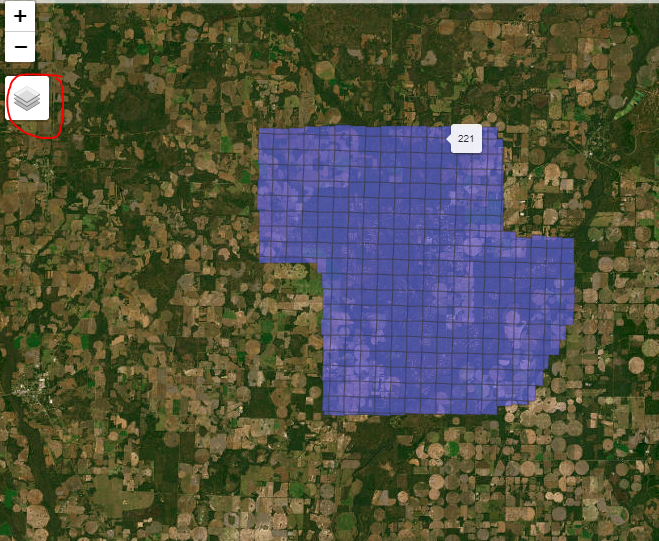
It can also be really useful to view the LAScatalog using mapview. This may require installation of the mapview package. You can also use the Layers button (red circle) to add a basemap.
plot(ctg, mapview = TRUE)

This data covers a very large area, over 300 km2 and contains over 5 billion lidar returns. Each tile represents a single .laz file as it is stored on your disk. The tiles allow us to access a small portion of the data at once.
Important Note: The LAScatalog object does not actually load the data into R. instead it just represents a map of where all the data is located. It is unlikely you can load all of the data at once anyway. So next we will define how we want to divide the data into chunks.
The data is already in 1000 × 1000 m files. But that does not mean we necessarily have to stick with these pre-defined boundaries. The LAScatalog object gives us a very convient way to define chunks however we like. We can also set a buffer in the way we would like, and we can even set filters like the ones you learned about in the last module. That way, when data is read in, you only load the data you need.
You can set options with the opt_filter, opt_chunksize, and opt_chunk_buffer options.
# Let's make the chunks bigger!
opt_chunk_size(ctg) = 2000

# give each chunk a 10 m buffer
opt_chunk_buffer(ctg) = 10

# Choose the origin of where your chunks are drawn
# i like them to snap to round numbers, so start at (0,0).
opt_chunk_alignment(ctg) = c(0,0)

# let's thin data down to 0.5 m voxel
opt_filter(ctg) = '-thin_with_voxel 0.5'

# Now view your chunk pattern
plot(ctg, chunk_pattern = TRUE)
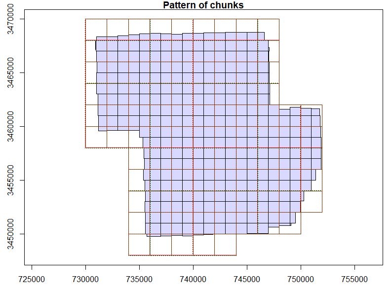
In the image below, the lavender squares still show how the original data is divided into tiles. However, the new larger black squares show the analytical chunks that you have defined. Here are some things to note:

LAScatalog object plotted with the chunk_pattern shown
- When we process data, the
lidRpackage will start with the bottom-left chunk, first, and work rightward, and then upward. - Each time it works on a chunk, it will automatically load the correct bits of each file for that chunk.
- It can quickly load just the portions you need for that chunk because you have already indexed the file!
- The hard to see red lines are actually slightly larger than the black squares. In addition to the 2000 × 2000 m tiles,
lidRwill also automatically load an extra 10 m buffer on each side. So, the tile that gets loaded will actually be 2020 × 2020 m.
Using the code above, define several different chunk sizes, buffers, and alignments so you get a better feel for how the LAScatalog chunk options work.
Next steps
Now you have all the tools you need to tackle a really big analysis. In the next module, you will put a lot of what you have learned together and create a digital elevation model for the entire 300 km22 area! In the next module you will learn to:
- Create a digital elevation model and stem map for a large area
- Divide a lidar dataset into many
chunksto process seperately - Deal with edge effects using the
catalog_mapfunction - Utilize parallel processing to speed up analyses with the
futurepackage - Combine all outputs into a single seamless product
Continue learning
- Module 1: Acquiring, loading, and viewing LiDAR data
- Module 2: Creating raster products from point clouds
- Module 3: Mapping trees from aerial LiDAR data
- Module 4: Putting it all together: Asking ecological questions
- Module 5: Speeding up your analyses: Reduced datasets
- Module 6: Speed up your analyses: Parallel processing with LAScatalog
- Module 7: Putting it all together (large-scale raster products)