Introduction and goals
In the last module, we covered how to load LiDAR data and generate a canopy height model. In this module we will learn how to automatically detect, map, and estimate the size of trees in an aerial LiDAR scene. By the end of this module, you should be able to:
- Use a canopy height model to identify tree locations
- Individually segment trees and estimate tree size
- Turn a LiDAR point cloud into a stem map
Pre-processing LiDAR data
You do not need any new additional LiDAR packages for this module, you can use the libraries we have already downloaded including lidR, lidRviewer, and terra.
Download this sample LiDAR dataset used in the previous modules. Load and de-noise the LAS object to prepare for analysis. If you need a refresher for how to load and de-noise, check the previous modules (Module 1: Acquiring, loading, and viewing LiDAR data).
library(lidR)
library(lidRviewer)
library(terra)

# Load example dataset above, or path to your data.
las = readLAS('NEON_D03_JERC_DP1_740000_3459000_classified_point_cloud.laz')
# or if you downloaded the reduced dataset instead
las = readLAS('NEON_D03_JERC_DP1_740000_3459000_classified_point_cloud-reduced.laz')

# Classify all isolated returns. Takes a few seconds
las = classify_noise(las, ivf(res = 3, n = 10))

# Filter out the noise
las = filter_poi(las, Classification != LASNOISE)

# The highest point value has a Z of 972.81. Keep only points below it.
max(las$Z)
las = filter_poi(las, Z < 970)
Create a canopy height model (CHM)
The first step in stem mapping with aerial LiDAR is to generate a canopy height model, as you did in the previous module (Module 2: Creating raster products from point clouds). The basic steps are to build a model of the canopy surface with the rasterize_canopy function, and subtract out the effects of elevation using the rasterize_terrain. For review, see the previous module (Module 2: Creating raster products from point clouds).
las = classify_ground(las, algorithm = csf()) #see `?csf` for more options
# This may take a little while. We'll learn how to 'thin' point clouds later
# You may get a warning that the points were already classified. That's because NEON data comes pre-classified. But that's not always the case!

# make a ditigal elevation model
dem = rasterize_terrain(las, res=1, algorithm=tin())
# OR you can also load the dem you created previously
# rast(dem, 'dem.tiff')

# Make a canopy surface model
csm = rasterize_canopy(las, algorithm = pitfree())

# Make a canopy height model by subtracting the csm from the dem
chm = csm - dem
Mapping tree locations
There are several methods for mapping trees and tree crowns from aerial LiDAR. One that seems to work well in longleaf pine forests is a method developed by Dalponte and Coomes (2016). The method uses the canopy height model, and searches in various windows to find local maximums that are characteristic of tree tops. Once tree tops are located, the algorithm searches the area around the tree tops and delineates the crowns that correspond by searching the area around the top, and eliminating low points from the ground or midstory.
Tree mapping will also require fine-tuning based on your specific forest, research question, and tolerance for error. Here we will use some basic parameters that seemed to work well for demonstration. Identifying trees can be done with the locate_trees function. This allows a manual option. See ?locate_trees. But you can also automate the process by searching via a local maximum function (lmf()). This function requres two parameters a search window size (ws) and a minimum tree height (hmin). We will start with a focus on large trees hmin = 10, and Silva et al. 2016 recommend a search radius of ~60% of tree height, so we’ll set ws = 6.
Let’s also plot and view this. You can layer the plot function by adding the argument add = TRUE. We’ll set the plot character to a solid circle (pch = 16) and shrink the size of the points using the character expansion option (cex = 0.1)
treetops = locate_trees(chm, lmf(ws = 6, hmin=10))

plot(chm)
plot(treetops$geometry, add = TRUE, pch = 16, cex = 0.2)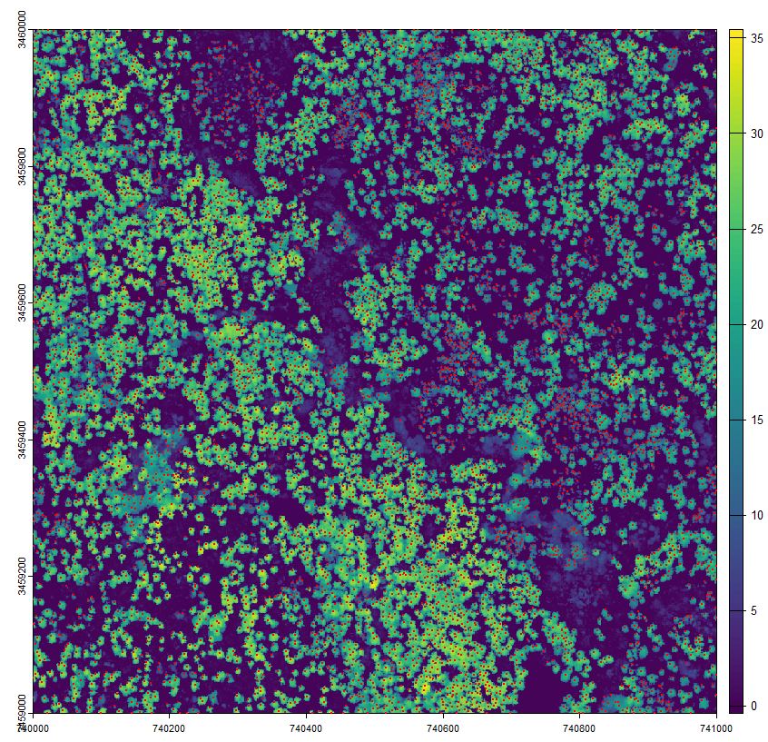
lmf() function in lidR package.Next we will implement the Dalponte and Coomes (2016) canopy delineation algorithm to identify the crown area for each tree.
#first define the algorithm..
# Here I multiply chm by 1 (this just makes sure chm is loaded into meory)
# it may not be required if you followed the steps straight through
# Also, you may get an error here about the 'future' package. You may need to first install it if you don't have it already. We will use the future package later to help with parallel processing.
install.packages('future')
crown_delineation_algorithm = dalponte2016(chm*1, treetops, th_tree = 2)

# Next we will execute it..
crown_raster = crown_delineation_algorithm()

# And convert it to polygons
crowns = as.polygons(crown_raster)

# plot and make sure there are plenty of colors to tell the crowns apart
par(mfrow = c(1,2))
plot(crowns, col=pastel.colors(8000))
plot(chm); plot(crowns, border=grey(0.5), add = TRUE)

# convert treetops to vect object and write to disk
writeVector(vect(treetops), 'treetops.shp')
writeVector(crowns, 'crowns.shp')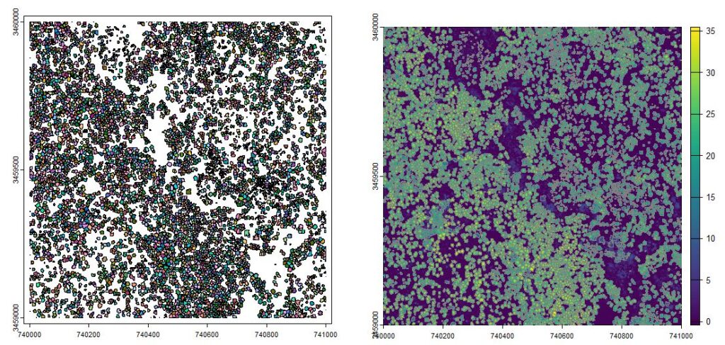
dalponte2016 method. Right. Delineated crowns overlaid on a 1-m resolution canopy height model.Stand characteristics
With aerial LiDAR, we don’t know the exact DBH of trees, but we can make some basic summaries of tree density, height distributions, and crown size distribution by examining the crowns object. To process the polygon of tree crowns, you may find the simple features sf package useful. Go ahead and install it.
install.packages('sf')
library(sf)
# Find the number of crowns delineated
n_trees = nrow(crowns)
# Calculate the area of the scene. [Product of the resoultion (1x1)] * [product of the dimensions (1000 x 1000)]
scene_area_m2 = prod(res(chm)) * prod(dim(chm))
scene_area_ha = scene_area_ha = scene_area_m2 / 10000
# Calculate tree density
print(n_trees/scene_area_ha) # There are ~68 trees per ha in the scene
# get area and radius of delineated crowns
crowns_sf = st_as_sf(crowns) # convert to sf object
crowns_sf$crown_area = st_area(crowns_sf)
crowns_sf$crown_radius = sqrt(crowns_sf$crown_area/pi)
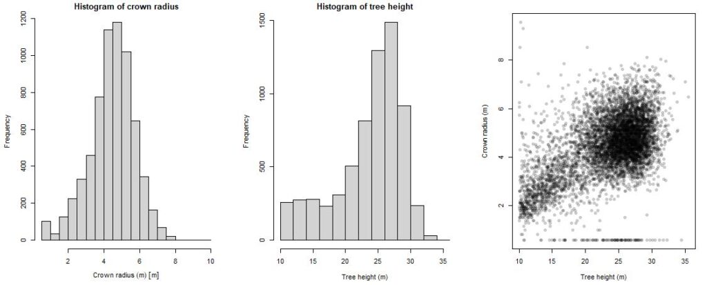
# Make histograms of tree heights and crown area
par(mfrow = c(1,3), mar=c(4,4,2,2)) # make a 1x3 panel plot
hist(crowns_sf$crown_radius, main='Histogram of crown radius', xlab='Crown radius (m)')
hist(treetops$Z, main = 'Histogram of tree height', xlab='Tree height (m)')
plot(crowns_sf$crown_radius ~ treetops$Z, xlab='Tree height (m)',
ylab='Crown radius (m)', pch=16, col='#00000033')
# the color setting #00000033 creates black plot point (000000) with a -33 level transparency
# Read more about hex color codes to learn more.
# https://www.pluralsight.com/resources/blog/upskilling/understanding-hexadecimal-colors-simple
Predicting diameter distribution
If you know how tree size (dbh) is related to tree heights, you can also make some estimates of diameter distribution. Note that this scene contains several species. We know that Pinus palustris dominates the uplands, but many different hardwood species dominate the low-lying areas. Here, we assume a single species relationship for demonstration purposes.
Gonzalez-Benecke et al. 2014 reports a relationship between longleaf pine height (𝐻) and diameter at breast height (𝑑𝑏ℎ) based on the parameters 𝑎1, 𝑎2, and 𝑎3.
H−1.37=exp(a1+a2∗dbh^a3)
Rerranging gives:
dbh=[loge(H−1.37)−a1)/a2]^(1/a3)
where
a1 = 3.773937
a2 = −7.844121
a3 = −0.710479
We can use this information to estimate the diameter of the delineated trees and create a diameter distribution for the scene. We know that not all the trees in the scene are longleaf pine, but for demonstration, let’s use this equation on everything.
#set parameters from Gonzalez-Benecke
a1 = 3.773937
a2 = -7.844121
a3 = -0.710479
# estimate dbh from tree heights stored in `treetops$Z`
dbh_cm = ((log(treetops$Z - 1.37) - a1) / a2 ) ^ (1/a3)

par(mfrow = c(1,2))
hist(dbh_cm, xlab = 'DBH (cm)', main='Histogram of tree diameters')
plot(treetops$Z ~ dbh_cm, xlab='Estimated dbh (cm)', ylab='Estimated height (m)')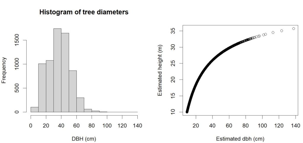
Next steps
Now you have taken a LiDAR scene and extracted data on thousands of trees. Although it is not as precise as field data, the trade off in extent and sample size may be useful for expanding your research to spatial scales that you could never hope to reach with standard field-based methods.
In the next module, you’ll learn to take some of the basic ecological data you’ve collected on elevation, tree size, and locations, and answer an ecological question.
The next module will cover:
- Extracting information from raster data of elevation and canopy height
- Extracting information on canopy size
- Associating information on elevation, canopy size, and tree height from individual trees.
- Testing some basic statistical models using information extracted from LiDAR.
Continue learning
- Module 1: Acquiring, loading, and viewing LiDAR data
- Module 2: Creating raster products from point clouds
- Module 3: Mapping trees from aerial LiDAR data
- Module 4: Putting it all together: Asking ecological questions
- Module 5: Speeding up your analyses: Reduced datasets
- Module 6: Speed up your analyses: Parallel processing with LAScatalog
- Module 7: Putting it all together (large-scale raster products)