Introduction

This collection of training modules is designed to get you started with basic LiDAR analysis for natural resources and forest ecology using R. It is primarily meant to help my students and staff get oriented to LiDAR analyses. By sharing it online, I am hoping others find it useful. These modules assume that you have a basic understanding of the R programming language, and some experience installing packages, manipulating data, and writing basic functions. By the time you finish this module you should be able to:

• Module 1: Acquiring, loading, and viewing LiDAR data
• Module 2: Creating raster products from point clouds
• Module 3: Mapping trees from aerial LiDAR data
• Module 4: Putting it all together: Asking ecological questions
• Module 5: Speeding up your analyses: Reduced datasets
• Module 6: Speed up your analyses: Parallel processing with LAScatalog
• Module 7: Putting it all together (large-scale raster products)

Module 1: Acquiring, loading, and viewing LiDAR data

Introduction and goals

Before getting started with LiDAR analyes, it is useful to know about different sources of LiDAR data, as well as how to load and view it in R. By the time you finish this module you should be able to:

• Download LiDAR data from public repositories
• Read *.las and *.laz files into R using the lidR package.
• Filter noise from LiDAR scenes
• Interactively plot and view LiDAR scenses by attributes.

Using R and RStudio

This tutorial assumes you have a basic understanding of using R, RStudio, and mastery of basic R commands. The following tutorials were built and tested using RStudio version 2024.09.0 running R version 4.4.0 on a Windows PC.

If you are using R for the first time, you may want to start with the following resources before completing the tutorial:

1. 15 min video: R programming for absolute beginners
2. “Basic Basics” tutorials: Unit 1: Basic Basics | R-Ladies Sydney
3. 40 Chapters: Comprehensive Introduction to R 

Downloading R packages

You will need several packages to get started. Some are mandatory, others are optional. The basic packages are available through the CRAN repository. However, because LiDAR technology is rapidly developing, some must be downloaded using their development version through GitHub.

• lidR: This package forms the foundation of LiDAR analyses in R and has many helpful functions for loading, viewing, and processing LiDAR data. In the more advanced modules, we will walk through using the LAScatalog functions for processing very large datasets using parallel computing.
• lidRviewer: Because LiDAR scenes can be so large, it can be slow to view them using the built in plot and rgl functions in R. The lidRviewer package provides a backend for quicker viewing. As of this writing, it is not available for my version of R 4.3.3 so we we will use the development version of lidRviewer from GitHub. Windows users: installing lidRviewer requires you to download an SDL library. See the instructions located at the github page for lidRviewer, and I have the code shown below. MacOS users: I have learned that it is not available for MacOS. You can still complete the modules without the lidRviewer package. Just leave off the backend='lidRviewer' from the plot() commands. It will plot more slowly using the rgl device, so only try this on small datasets.

Setting working directory and installing required packages

Create a new folder in a convenient location. For this example, we will create a folder called myLidar on the Windows Desktop: C:\Users\jeffery.cannon\Desktop\myLiDAR\ This will be our “working directory” where all inputs and outputs for the project will be saved.

Once you’ve opened RStudio start by setting the working directory to the folder you just created. You can do this by running the following command in the Console or from a new script.

setwd("C:/Users/jeffery.cannon/Desktop/myLiDAR")

Note that some programs are picky about which way the / leans.

Now you can install the packages that will be required. The lidR has many other packages that it depends on. These will also be installed, so you’ll se a wall of red text swirl by as they are installed.

# install CRAN packages if you haven't already
install.packages('lidR')

# install lidRviewer specified repository
install.packages('lidRviewer', repos = c('https://r-lidar.r-universe.dev'))

We will also install the lidRviewer package. It is not an official CRAN package and is trickier to install. First use the source() command below to load the sdl package.

LiDAR data sources

1. Download this sample LiDAR dataset to get start practicing right away with no fuss. This data will form the basis of the first four modules of this tutorial. I have learned some users with lower RAM resources have issues with the 150 MB dataset. You can also downloaded this reduced LiDAR dataset instead.
2. The USGS 3D Elevation Program (3DEP) provides LiDAR data coverage for large portions of the continental US, Puerto Rico, and the US Virgin Islands. Coverage is lower for Alaska and Hawaii. LidDAR acquisitions for the state of Georgia were completed over the years of 2019-2021 by USGS 3DEP.
3. For ecological research, you will find repeated LiDAR acquisitions at select sites of the National Ecological Observatory Network (NEON). LiDAR data from NEON is available between 2018 to present–approximately annually–at dozens of sites in the network. The sample data we are using comes from a section of the 2023 dataset from the JERC (Jones Center at Ichauway) longleaf pine ecosysetem in Newton, Georgia. We will return to this entire dataset in Module 5: Speeding up your analyses: Reduced datasets .

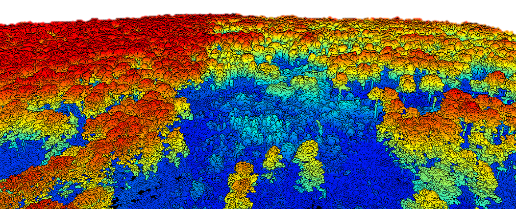
Sample LiDAR dataset from longleaf pine woodland in southwest Georgia as shown in the lidRviewer package

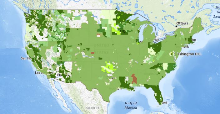
Publicly available LiDAR data available via USGS 3D Elevation Program.

Loading LiDAR data into R

Loading and viewing data in R is made simple with built-in functions in the lidR package. The typically large size of LiDAR data can create challenges for viewing them. You can use the lidRviewer package to view LiDAR data. An unfortunate downside is that it halts other R operations while you are viewing. Another option is to subset the data which we will cover in Module 5: Speeding up your analyses: Reduced datasets. You can also view point clouds in the specialized OpenSource Software Cloud Compare.

LiDAR data comes as a *.las file type which is uncompressed or *.laz which is a compressed version. You will also see *.lax files. These are index files which can greatly speed up your processing. We will cover indexing in Module 5: Speeding up your analyses: Reduced datasets. Less commonly you may also encounter raw point clouds in text formats (e.g., *.txt or *.xyz).

Read in and view data

# load the lidR library
library(lidR)
library(lidRviewer)

# Load example dataset above, or path to your data.
las = readLAS('NEON_D03_JERC_DP1_740000_3459000_classified_point_cloud.laz')

# or if you downloaded the reduced dataset instead
las = readLAS('NEON_D03_JERC_DP1_740000_3459000_classified_point_cloud-reduced.laz')

# plot using lidRviewer
view(las)

# with the viewer OPEN, press z on your keyboard
# This will color the points based on height (z-value)
# close the window when you are finished

Filtering out noise

You will notice that there is some noise in the dataset. There are some extraneous points that occur very high above or below the scene. Some noise is inevitable due to reflections, smoke and particulates, or even birds. You will need to filter these out. WIth the viewing window open, you can color the points based on their height (z-value) by pressing the z key on your keyboard.

The lidR package has functions to help filter out noise. It searches for returns that are far from neighbors ivf() the isolated voxel filter. Here, we filter all points where there is no more than n = 10 lidar returns within a resolution of 3 m. We then filter out the points of interest that are not classifid as noise. Note the variable LASNOISE = 18.

# Classify all isolated returns. Takes a few minutes
las = classify_noise(las, ivf(res = 3, n = 10))

# The classify_noise function sets
# Classification = 18 (LASNOISE = 18)
las = filter_poi(las, Classification != LASNOISE)
view(las)

# You can use trial and error to adjust parameters or
# base the parameters on knowledge of the scan
# This scene still has some pesky noise that must be in a cluster. Let's delete it manually.
# Take a look at the highest point, and filter out data below it
max(las$Z) #which Z value has the maximum value.

# The highest point value has a Z of 972.812. Keep only points below it.
las = filter_poi(las, Z < 970)

# View it now
view(las)
# Press the z-key to view it colored by height

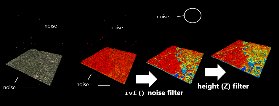
Sample data showing results of noise and height filter

You saw in the last section that the las object had the attribute Z corresponding in this case to elevation. There are many other attributes we can also see. Check the las@data slot to see what all the data is stored for points. You can color point clouds by some of these traits. Here are some useful ones to know.

colnames(las@data)

# View the help file for lidRviewer::view() to see how to change color displays
?view

# press r, g, or b, to view color with RGB

# press z to color with z value (elevation above see level)

# press i to color with lidar return intensity
# Ground and trunks have a higher intensity than vegetation

# press c to color with point classification (if available)
# The example point cloud is already classified. We'll learn to classify points later
# Green = tall vegetation, yellow = short vegetation, blue = ground

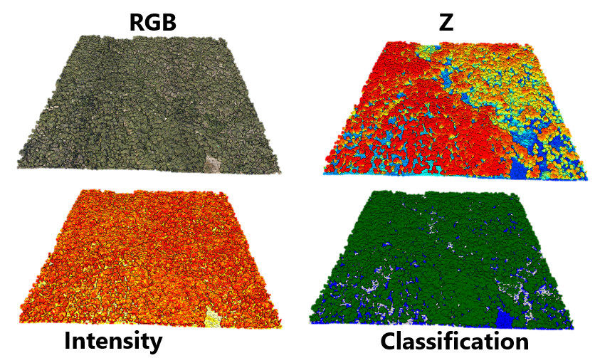
Sample plot illustrating coloring by various attributes associated with the lidar data using lidRviewer

Next steps

Now you can download, de-noise, and view basic LiDAR data. Now that we have the basics., we will start extracting useful information from the point clouds. In the next module, you will learn how to

• generate a digital elevation model (raster) from LiDAR data
• generate a canopy height model (raster) from LiDAR data

Continue learning

• Module 1: Acquiring, loading, and viewing LiDAR data
• Module 2: Creating raster products from point clouds
• Module 3: Mapping trees from aerial LiDAR data
• Module 4: Putting it all together: Asking ecological questions
• Module 5: Speeding up your analyses: Reduced datasets
• Module 6: Speed up your analyses: Parallel processing with LAScatalog
• Module 7: Putting it all together (large-scale raster products)