Savannah Rascon, Seasonal Technician

What is LiDAR? 

LiDAR, or Light Detection and Ranging, is an emerging remote sensing technology that can be applied to research in forested environments to construct a three-dimensional model of a forest stand. In Landscape Ecology Lab at the Jones Center, we are constantly brainstorming new ways to apply this technology to improve conservation and restoration efforts. Traditional methods for gathering data on tree characteristics, such as tree height and DBH, are labor intensive and time consuming. Moreover, some attributes like crown architecture and crown symmetry can be subjective and difficult to quantify in the field.  

Aerial LiDAR is collected through a scanner mounted on a drone or plane and can quickly gather data over vast areas of land. Aerial LiDAR produces 3D point clouds that can be used to estimate a plethora of forest characteristics, from tree height to crown size and stand density. Terrestrial LiDAR units, on the other hand, are carried by a single person in the field and can capture fine-scale details on individual trees including trunk taper and canopy architecture traits.  While aerial LiDAR produces coarser resolution data than terrestrial LiDAR, it provides the crucial benefit of collecting information at very large scales. 

Developing Functions in R to Extract Stand Attributes  

I was tasked with using aerial LiDAR to monitor changes in forest structure in a 30-year-old longleaf pine stand after thinning. After completing our lab’s online tutorials for getting started with LiDAR, I was able to develop an R script that can input LiDAR point clouds in the form of .las files and produce a visual map of tree crowns as well as estimates of tree- and stand-level attributes such as crown area and tree density. The intention is to use this code to rapidly collect information on stand structure after forest operations. The following is a tutorial explaining how to use the resulting code. For this example, I will be using data from a planted longleaf pine stand at the Jones Center at Ichauway that was thinned in 2020 (31.172°, -84.464°). I have supplied LiDAR data from before and after the thinning to demonstrate how it can be used to identify modifications in stand structural characteristics.  

Tutorial 

Setting a working directory, file paths, and parameters 

This tutorial assumes a basic understanding of R, such as the initial installation of R, opening an R script and the purpose of setting a working directory.  

Begin by setting your working directory to a convenient location.  

setwd('C:/Users/YourUsername/YourFolderName') 

Then, load your file paths and set parameters based on your needs. This tutorial provides potential parameter settings, but these can and should be adjusted for the specifications of the stand of interest. Particularly, parameters such as height_minimum, the minimum height required for identification of an individual tree, should be considered. We have experimented with noise filters and found these settings to best remove noise in our LiDAR point clouds. 

# set file paths 
las_path_PRE = 'C:/Users/YourUsername/YourFolderName/YourFilePRE.las' 

las_path_POST = 'C:/Users/YourUsername/YourFolderName/YourFilePOST.las' 
 
# Noise filter resolution in m^3  
resolution <- 2 

# Noise threshold  
noise <- 10  

# Window size for local maximum function 
window_size <- 7 

height_minimum <- 10 

Running functions to calculate tree- and stand-level metrics 

Now let’s load in the functions. We’ll start by creating a function called “las_path_to_chm()”. This function takes a .las file as an input, and outputs a canopy height model as a raster. The parameters ‘resolution’ and ‘noise’ must be set. Resolution refers to the resolution in meters of the 3D voxel search area for noise points. The noise parameter refers to the minimum number of points required to be found within a voxel for it to not be considered noise. 

# this function reads in a .las file, filters out noise, and creates a canopy height model
las_path_to_chm = function(path, resolution = 2, noise = 10) {
     las <- lidR::readLAS(path)
     las <- lidR::classify_noise(las, lidR::ivf(res = resolution, n = noise))
     las <- lidR::filter_poi(las, Classification != lidR::LASNOISE)
     las <- lidR::classify_ground(las, lidR::csf())
     dem <- lidR::rasterize_terrain(las, res = 1, lidR::tin())
     csm <- lidR::rasterize_canopy(las, res= 1, lidR::pitfree())
     chm <- csm - dem
     return(chm)
}

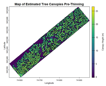
You can see the result of the canopy height model in the figure below. Next, we will use the canopy height model to produce several useful outputs. The first is a map of the study area that denotes tree locations by finding local maxima in the canopy height model. We will also use a function capable of carving out boundaries of individual tree crowns. These objects are plotted as a black dot for tree locations and tree crown boundaries are shown as a black outline. We will also output a list containing a shapefile with estimates of crown area and radius, as well as a shapefile with tree height and location information. 

# This function reads in a canopy height model, and estimates treetop locations and crown boundaries 
chm_to_crowns = function(chm, window_size, height_minimum, plot=TRUE) { 
     treetops <- lidR::locate_trees(chm, lidR::lmf(ws = window_size, hmin = height_minimum)) 
     crown_algorithm <- lidR::dalponte2016(chm, treetops, th_tree = 2) 
     crown_raster <- crown_algorithm() 
     crowns <- terra::as.polygons(crown_raster) 
     crowns_sf <- sf::st_as_sf(crowns) # convert to sf object 
     crowns_sf$crown_area <- terra::expanse(crowns) 
     crowns_sf$crown_radius <- sqrt(crowns_sf$crown_area/pi) 
     if(plot) { 
          terra::plot(chm, main = "Map of Estimated Tree Canopies", xlab = "Longitude", ylab = "Latitude",mar = c(4,1,4,0.5)) 
          mtext("Canopy Height (m)", side = 4, line = -5, cex = .8) 
          plot(crowns_sf, add=TRUE, col=NA) 
          plot(treetops$geometry, add = TRUE, pch = 16, cex = 0.2) 
     } 
     return(list(crowns=crowns_sf, trees=treetops)) 
} 

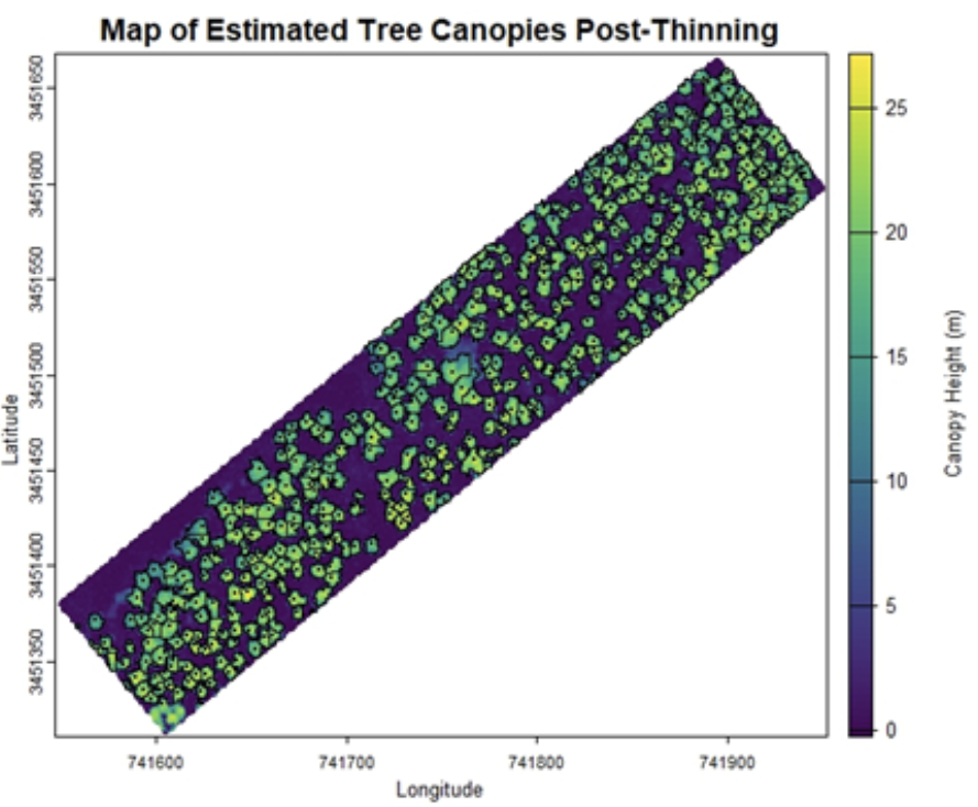
Below are the resulting graphs for the pre-thinning and post-thinning data at the example site. The differences in canopy openness are visually apparent, but let’s run two more functions to finish gathering some stand attributes. 

From here we’ll take our two shapefiles and run calculations of DBH and basal area. We’ll also extract X and Y coordinates for each tree detected, as well as assign each tree an ID number. We will then reorder the columns of the shapefile to organize our data. The output will be a cleaned data frame that encapsulates tree-level characteristics, such as crown area and basal area for each individual tree. Tree trunks are difficult to measure with aerial LiDAR because they are obscured by the tree crowns. Luckily, trunk diameter of longleaf pine can be predicted fairly accurately from tree height (at least for young trees) and this is much easier to measure aerial LiDAR. Once we’ve measured individual tree crowns, we can use them to estimate tree size. 

# this function inputs the crowns_output and calculates DBH, basal area, and
# coordinates and outputs a dataframe
crowns_to_dataframe = function(crowns_output) {

     crowns = crowns_output$crowns
     trees = crowns_output$trees
     # DBH allometric parameter following Gonzalez-Benacke
     dbh_cm <- ((log(trees$Z - 1.37)- 3.773937) / -7.844121) ^ (1/-0.710479)
     ba_tree <- pi*((dbh_cm/200)^2)location_coordinates <- sf::st_coordinates(trees$geometry) 

     location_coordinates <- as.data.frame(location_coordinates) 
     crowns$X <- location_coordinates$X 
     crowns$Y <- location_coordinates$Y 
     crowns$Height <- trees$Z 
     crowns$DBH <- dbh_cm 
     crowns$TreeID <- trees$treeID 
     crowns$Individual_BA <- ba_tree 
     Tree_Level <- crowns[, c(9, 5, 6, 2, 7, 8, 4, 3, 10)] 

     return(Tree_Level)
}

Finally, we will use the data frame exported from the previous function containing tree-level information to calculate stand metrics including stand density, quadratic mean diameter, and basal area of the stand. 

# gather stand characteristics from tree measurements 
stand_inventory_function <- function(Tree_Level, chm = las_path_to_chm_output) { 
     tree_count <- nrow(Tree_Level) 
     total_ba <- sum(Tree_Level$Individual_BA) 
     area_m2 <- sum(!is.na(chm[])) * prod(terra::res(chm)) 
     area_ha <- area_m2/10000 
     basal_area <- total_ba/area_ha 
     trees_per_ha <- tree_count/area_ha 
     qmd <- sqrt((basal_area/trees_per_ha)/0.00007854) 

     Stand_Level <- data.frame(1) 
     Stand_Level$Tree_Count <- tree_count 
     Stand_Level$Tree_Density <- trees_per_ha 
     Stand_Level$Basal_Area <- basal_area 
     Stand_Level$Quadratic_Mean_Diameter <- qmd 
     return(Stand_Level) 
} 

Below is an example of the workflow for the series of functions, with tree_level and stand_level data frames as the final products.  

# Pre-Thinning 
chm_PRE <- las_path_to_chm(las_path_PRE) 
crowns_PRE <- chm_to_crowns(chm_PRE, window_size = window_size, height_minimum = height_minimum, plot = TRUE) 
tree_level_pre <- crowns_to_dataframe(crowns_PRE) 
stand_level_pre <- stand_inventory_function(tree_level_pre, chm = chm_PRE) 

# Post-Thinning 
chm_POST <- las_path_to_chm(las_path_POST) 
crowns_POST <- chm_to_crowns(chm_POST, window_size = window_size, height_minimum = height_minimum, plot = TRUE) 
tree_level_post <- crowns_to_dataframe(crowns_POST) 
stand_level_post <- stand_inventory_function(tree_level_post, chm = chm_POST)

Applying LiDAR Data to Ecological Forestry 

At the Jones Center at Ichauway, a major management objective is the conservation and growth of longleaf pine (Pinus palustris). Longleaf pine once covered vast swaths of the southeastern United States, yet today it covers only 5% of its range prior to EuroAmerican colonization. Management of longleaf pine on Ichauway follows the principles of ecological forestry, under which timber is sustainably managed in such a way as to prioritize the health and resilience of the ecosystem as a whole. This means that habitat for wildlife, natural regeneration, sustainable tree populations, continuation of prescribed burning, and promotion of a healthy native understory are all taken into account alongside financial considerations. At the Jones Center, timber is harvested following an individual-tree selection strategy called the Stoddard-Neel Approach. The Stoddard-Neel Approach utilizes the thinking of ecological forestry by selecting individual trees for harvest with the objective of promoting a multi-aged stand that maintains the structure and organic components needed to support native flora and fauna. Individual trees are selected for harvest based on a combination of characteristics such as the presence of burn scars, insect damage, crown symmetry, the quality and quantity of the needles for fuel input, the local density of trees and natural regeneration, and the structure of light reaching the forest floor. A commonly implemented strategy is to introduce gaps in the canopy by removing several trees within a particular area. This is meant to mimic natural disturbances such as hurricanes and tornadoes, which often create canopy openings. The intention is to support regeneration by reducing competition for light and growing space.  

Mapping the outcome of a thinning operation is of interest to researchers and land managers to track the structure of gaps created and determine whether or not the intended response, such as increased regeneration, is observed. However, the time consuming and labor intense nature of on the ground field work by technicians makes monitoring changes in stands over time challenging. Therefore, we are eager to apply LiDAR to collecting information on tree growth and stand structure as they response to natural and manmade disturbances.  

In this example, the changes in canopy openness are apparent. The data frames produced for these datasets estimate that in 2019, before the most recent thinning operation, there were 571 trees in this stand with a tree density of ~141 trees per hectare (57 trees per acre). Comparatively, the produced data frames for the 2021 post-thinning data estimated that the stand retained 447 trees and had a reduced tree density of ~110 trees per hectare (45 trees per acre). In future years, this script could be run again on the same plot to determine if and when new recruitment appears within the gaps that were introduced. For this example, the script detects trees with a minimum height of 10 meters, but this could be changed to scan for trees with a shorter minimum height. As mentioned at the beginning of the tutorial, land managers interested in monitoring regeneration could calibrate the tree height minimum parameter to detect younger, shorter trees. Ultimately, this code is a promising steppingstone towards harnessing the potential of LiDAR data to monitor stand change and growth over time.