Introduction and goals
By now you have derived useful information from the LiDAR scene, it is time to use the data to ask some ecological questions. In this module, you will learn how to :
- Extract information from raster data of elevation and canopy height
- Extract information on canopy size
- Associate information on elevation, canopy size, and tree height from individual trees.
- Build a basic statistical model using information extracted from LiDAR.
To keep it simple, we will start by asking some simple ecological questions We will ask:
How do tree height and canopy change with elevation?
In our scene, upland areas usually consist of sandy, well drained soils dominated by longleaf pine. The bottomlands are richer floodplains that host a diverse array of harwood species such as live oak. Longleaf pine (Pinus palustris) is very tall with a compact crown, whereas live oak (Quercus virginiana) is a shorter species with a sprawling wide canopy. Can we detect these differences in our elevational gradient?
From our earlier analyses we already have the information to answer this question. We will need to
- Extract the elevation (from the digital elevation model) to every tree location
- Extract the canopy size (from the canopy vector) for every tree location
- Extract the tree height (from the canopy height model) for every tree location
Preparing the data
If you have not yet done so, use the LiDAR data to make a (1) digital elevation model, (2) a canopy height model, (3) a stem map and (4) crown delineation feature. Check the previous tutorial (Module 3: Mapping trees from aerial LiDAR data) if you need a refresher.
# libraries
library(lidR)
library(terra)

# Load and denoise LiDAR data.
las = readLAS('NEON_D03_JERC_DP1_740000_3459000_classified_point_cloud.laz')
las = classify_noise(las, ivf(res = 3, n = 10))
las = filter_poi(las, Classification != LASNOISE)
las = filter_poi(las, Z < 970)

# Classify ground points, create a dem and chm
las = classify_noise(las, ivf(res = 3, n = 10))
las = filter_poi(las, Classification != LASNOISE)
las = classify_ground(las, algorithm = csf()) #see `?csf` for more options
dem = rasterize_terrain(las, res=1, algorithm=tin())
csm = rasterize_canopy(las, algorithm = pitfree())
chm = csm - dem

# Generate a stem map and crown delineation feature
treetops = locate_trees(chm, lmf(ws = 6, hmin=10))
crown_delineation_algorithm = dalponte2016(chm, treetops, th_tree = 2)
crown_raster = crown_delineation_algorithm()
crowns = as.polygons(crown_raster)

# Check out the data...
plot(chm)
plot(crowns, add=TRUE)
Extracting elevation
Now we need to get the elevation for all 6,847 trees in our dataset! To do this, we simply need to obtain the elevation value underneath each tree location. The terra package makes this easy with the the extract function.
# Use the extract function, (Note i added the `terra::extract(...)` prefix to avoid conflict with another package, you may just be able to use `extract(...))
terra::extract(dem, treetops) # they are stored in a column titled Z

treetops$elevation = terra::extract(dem, treetops)$Z

par(mfrow = c(1,2)) # make a 1 x 2 panel window
plot(dem)
plot(treetops$geometry, add = TRUE, pch = 16, cex = 0.1)
hist(treetops$elevation)
Extracting tree heights and crown areas
Now we need to extract the properties of the trees themselves. You can extract the tree heights the same as elevation, but this time use the canopy height model as the input layer. To get the area of crowns, we need to know the area of each feature in the crown polygon. You can get that with the expanse function from terra.
# extract tree heights from the chm
treetops$ht_m = extract(chm, treetops)$Z

#extract area of crowns in units of the coordinate system
treetops$area_m2 = expanse(crowns)

par(mfrow = c(1,2))
hist(treetops$ht_m)
hist(treetops$area_m2)$Z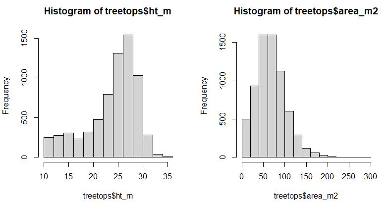
How does tree height change with elevation?
To adress how tree height changes with elevation, we can use the data we collected on all 6,847 trees. Please note that for demonstration purposes, we will take liberties with statistical assumptions.
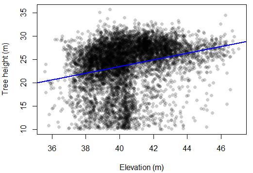
To test the hypothesis that tree height is associated with elevation, we can use a linear model using the lm function with ht_m as a response variable and elevation as a predictor variable. We can view the results of the model with the summary function, and plot the data with a best fit line.
# Make a regression of height versus elevation
height_model = lm(ht_m ~ elevation, data = treetops)

# Check the model (we are certainly violating assumptions here...)
summary(height_model)

# View the scatter plot
plot(treetops$ht_m ~ treetops$elevation, pch=16, col='#00000033',
     xlab = 'Elevation (m)', ylab= 'Tree height (m)')
# plot character = 16 (solid circle)
# col = black (hex code #000000) with some transparency (33), FF for no transparency

# Add best fit line
abline(height_model, col='blue', lwd=2) #line width = 2
Model output
Call:
lm(formula = ht_m ~ elevation, data = treetops)

Residuals:
    Min      1Q  Median      3Q     Max
-16.671  -1.949   1.208   3.416  12.614

Coefficients:
            Estimate Std. Error t value Pr(>|t|)
(Intercept)  -5.0800     1.2841  -3.956  7.7e-05 ***
elevation     0.7151     0.0317  22.559  < 2e-16 ***
---
Signif. codes:  0 ‘***’ 0.001 ‘**’ 0.01 ‘*’ 0.05 ‘.’ 0.1 ‘ ’ 1

Residual standard error: 4.95 on 6845 degrees of freedom
Multiple R-squared:  0.0692,    Adjusted R-squared:  0.06906
F-statistic: 508.9 on 1 and 6845 DF,  p-value: < 2.2e-16
There appears to be a clear trend of taller trees in the uplands from this data. For every 1 m that elevation increases, tree height increases by ~2 m. Note that this seems to be driven, in part, by many small trees that are in the 38-40 m range.
How does tree crown area change with elevation?
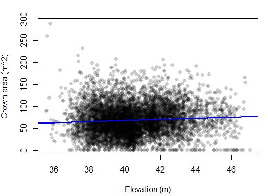
To address how canopy size changes with elevation, we can repeat the process, this time using area_m2 as a response variable and elevation as a predictor variable. Once again, we view the results of the model with the summary function, and plot the data with a best fit line.
# Make a regression of height versus elevation
crown_model = lm(area_m2 ~ elevation, data = treetops)

# Check the model (we are certainly violating assumptions here...)
summary(crown_model)

# View the scatter plot
plot(area_m2 ~ elevation, data=treetops, pch=16, col='#00000033',
     xlab = 'Elevation (m)', ylab= 'Crown area (m^2)')
# plot character = 16 (solid circle)
# col = black (hex code #000000) with some transparency (33), FF for no transparency

# Add best fit line
abline(crown_model, col='blue', lwd=2) #line width = 2
Model output
Call:
lm(formula = area_m2 ~ elevation, data = treetops)

Residuals:
    Min      1Q  Median      3Q     Max
-74.967 -23.047  -2.971  20.527 226.673

Coefficients:
            Estimate Std. Error t value Pr(>|t|)
(Intercept)  18.8161     8.8925   2.116   0.0344 *
elevation     1.2150     0.2195   5.535 3.23e-08 ***
---
Signif. codes:  0 ‘***’ 0.001 ‘**’ 0.01 ‘*’ 0.05 ‘.’ 0.1 ‘ ’ 1

Residual standard error: 34.28 on 6845 degrees of freedom
Multiple R-squared:  0.004456,  Adjusted R-squared:  0.00431
F-statistic: 30.64 on 1 and 6845 DF,  p-value: 3.229e-08
This effect appears more subtle. There is a slightly higher crown area in the higher elevations. We expected the opposite trend (large crowns from oaks in the lower elevation). Perhaps the same short trees in the 38-40 m elevation range are bringing the average down?
Of course we are violating all kinds of statistical assumptions here. The trees are close together, so the crown area and heights are non-independent. The residuals of the model are not normally distributed. But this is not a statistics class. We just want to learn how to extract data from LiDAR 🙂
Next steps
Now you have gone once through the entire process. You have started from raw LiDAR point clouds and processed them to answer basic ecological questions. Of course, we have only scratched the surface. Every day, there are new algorithims that you can use to extract useful information from LiDAR point clouds. Hopefully, you will also develop some of your own!
Although 1 km2 may seem like a large area compared to what you can achieve with field methods, it is quite small for an aerial LiDAR analysis. The real power comes from working with very large datasets. But before scaling up, you will need to learn some basic skills to help with large data.
In the next module, you will learn to:
- Create a spatial index to speed up loading partial datasets
- Subset a LiDAR scene to focus on a smaller area of interest
- Create a lower density point cloud when lower resolution data is acceptable
Continue learning
- Module 1: Acquiring, loading, and viewing LiDAR data
- Module 2: Creating raster products from point clouds
- Module 3: Mapping trees from aerial LiDAR data
- Module 4: Putting it all together: Asking ecological questions
- Module 5: Speeding up your analyses: Reduced datasets
- Module 6: Speed up your analyses: Parallel processing with LAScatalog
- Module 7: Putting it all together (large-scale raster products)