Happy New Year from the Aquatic Sciences Lab!
The lab celebrates our first-year anniversary this month and we are looking both backwards at a busy 2024 and forwards to an exciting 2025. We will be making our way to you at conferences and welcoming new lab members and graduate students (more to come soon!).
As we reflect on 2024, we look back on the year in rainfall. Maybe this becomes a recurring post around the beginning of the year? Maybe we evaluate a different measurement that we (or our collaborators) make continuously throughout the year? But for today…
Rainfall Wrapped!
The Jones Center collects rainfall in a few locations and in collaboration with various partners. Rainfall is collected by the Ecohydrology lab at climate stations and in various wetlands across the property. They use wetland rainfall collectors to precisely determine water budgets, which is a challenge for our many tiny (<5 ha) wetlands. Our collaborators at NEON collect rainfall at their installation. The Georgia Automated Environmental Monitoring Network (GAEMN) collects rainfall at a climate station on site for Baker County, Georgia. Finally, we partner with NOAA to maintain a climate station. So, when we need to pick rainfall, there are many options to choose from!
We will also use this post as an example of how to analyze rainfall data with R code.
For this exercise, we will use data from the GAEMN station. These data are collected every 15 minutes, so for an entire years’ worth of data, there are 35138 observations! We can make that an easier chunk by summing together rainfall for each day and creating a time-series for each day. Graphs showing rainfall are shown with rainfall ‘falling’ from the top of the graph towards the bottom; the formal name for a graph like this is a ‘hyetograph’.
First, we will load the necessary packages and data into R and make sure R interprets the first column as a date-time stamp.
# load packages
library(tidyverse)

# climate file directory
clim_files <- list.files('R:/aquatic_sciences/climate/2024/',
                         full.names = TRUE)

# load all files in that directory into a single object
df_2024 <- purrr::map_dfr(clim_files,
                   readr::read_csv)

# fix the date
df_2024$Date <- as.POSIXct(df_2024$Date,
                           '%m-%d-%Y %H:%M',
                           tz = 'America/New_York')

# sum up each day's rainfall
df_2024_daily <- df_2024 %>%
  dplyr::group_by(date = lubridate::date(Date)) %>%
  dplyr::summarise(daily_rain = sum(`Rain mm`,
                                    na.rm = TRUE)) %>%
  dplyr::filter(!is.na(date))

# take a peak
head(df_2024_daily)
## # A tibble: 6 × 2
## date daily_rain
## <date> <dbl>
## 1 2024-01-01 0
## 2 2024-01-02 0
## 3 2024-01-03 0.508
## 4 2024-01-04 0
## 5 2024-01-05 4.57
## 6 2024-01-06 24.6Daily Rainfall
fig_1 <- ggplot(df_2024_daily,
       aes(x = date,
           y = daily_rain))+
  geom_bar(stat = 'identity')+
  lims(y = c(125, 0))+
  labs(y = 'Rainfall (mm/day)',
       x = element_blank())+
  theme_classic()
fig_1
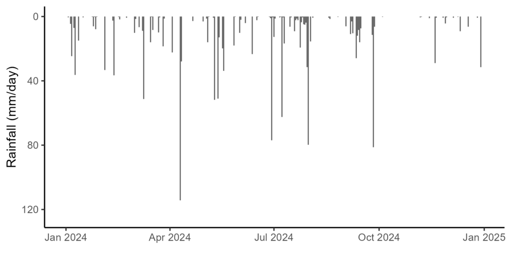
Next, we can calculate some values of interest for the year:
- The total annual rainfall for 2024 was 1377.916
- The wettest day of the year was 2024-04-10
- The number of days with 0 rainfall was 257 . That means there was 70% sunny days at Ichauway!
We can determine the length of continuous days with no rain and the length of days with continuous rain using the following code
rle <- rle(df_2024_daily$daily_rain)

rle_df <- data.frame(values = rle$values,
                     lengths = rle$lengths)

rle_df %>%
  filter(values == 0) %>%
  slice_max(lengths) %>%
  pull(lengths)
## [1] 32x <- df_2024_daily %>%
mutate(rained = ifelse(daily_rain > 0,
1,
0))
y <- rle(x$rained == 1)
data.frame(length = y$lengths,
values = y$values) %>%
filter(values == TRUE) %>%
slice_max(length) %>%
pull(length)## [1] 8Monthly Rainfall
To explore seasonality in rainfall, we can look at monthly rainfall
df_2024_month <- df_2024 %>%
  group_by(month = lubridate::month(Date,abbr = TRUE, label = TRUE)) %>%
  summarise(daily_rain = sum(`Rain mm`, na.rm = TRUE)) %>%
  filter(!is.na(month))
df_2024_month
## # A tibble: 12 × 2
## month daily_rain
## <ord> <dbl>
## 1 Jan 103.
## 2 Feb 75.2
## 3 Mar 133.
## 4 Apr 170.
## 5 May 206.
## 6 Jun 121.
## 7 Jul 265.
## 8 Aug 18.8
## 9 Sep 199.
## 10 Oct 0.254
## 11 Nov 37.1
## 12 Dec 48.8
fig_2 <- ggplot(data = df_2024_month,
aes(x = month))+
geom_bar(aes(y = daily_rain),
stat = 'identity')+
lims(y = c(300, 0))+
labs(x = element_blank(),
y = 'Rainfall (mm/month)')

The wettest month was July (265 mm), followed closely by May (206 mm). The driest months were October (0.25 mm) and August (19 mm). The data show a wetter period in the brief winter, spring, and early summer that yields to a drier summer and fall period.
Hurricane Helene
Let’s take a closer look at September. If we imagine a seasonal trend as described above, we might expect September to have been a drier month than the data show. We must remember that hurricanes are a common occurrence at Ichauway and across the SE US. And between September 24 – 26, Hurricane Helene ripped across the eastern edge of the property, with strong winds and rain. We can filter the dataset to explore rainfall during September and see if Hurricane Helene stands out.
df_2024_daily %>%
  filter(between(date, as.Date('2024-09-01'), as.Date('2024-10-01'))) %>%
  ggplot(.,
         aes(x = date,
             y = daily_rain))+
  geom_bar(stat = 'identity')+
  lims(y = c(100, 0))+
  labs(x = element_blank(),
       y = 'Rainfall (mm/day)')+
  annotate(geom = 'text',
           x = as.Date('2024-09-26'),
           y = 95,label = '*', size = 15)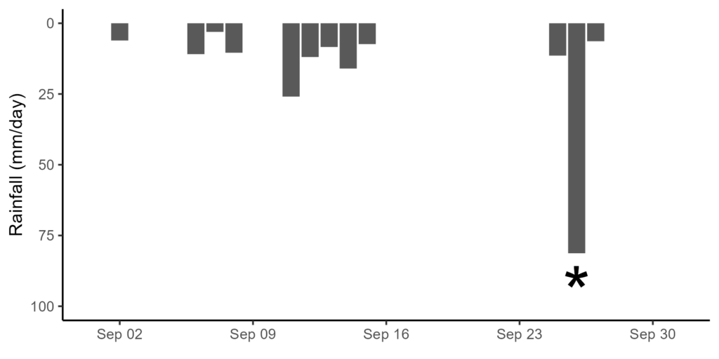
While we dodged the worst of the storm due to a late shift east-ward of the storm, our neighbors to the east received much stronger winds and more rain, not to omit mention of the flood damage across Georgia and western North Carolina.
Annual Rainfall
So, how does the rainfall during 2024 compare to other years? The GAEMN record has continuous records back to 2001 and we can compare rainfall during 2024 to each year in the past. We will have to do some data formatting to have the long-term data work with the 2024 data, and then we can combine into one single dataset.
# read in the long-term data
df <- readxl::read_excel('R:/temporary_storage/nmarzolf/GAEMN_weather_data_in_15min_standard.xlsx')

# make it easier to handle
short <- df %>%
  dplyr::select(Date, rain_in = `RainTotal (in)`) %>%
  dplyr::mutate(rain_cm = rain_in * 2.54)

# calculate daily cumulative rainfall
daily_cum_rain <- short %>%
  dplyr::group_by(date = lubridate::date(Date)) %>%
  dplyr::summarise(rain_tot_cm = sum(rain_cm, na.rm = TRUE))

# and annual cumulative rainfall
ann_cum_rain <- daily_cum_rain %>%
  dplyr::mutate(year = lubridate::year(date),
                jday = lubridate::yday(date)) %>%
  group_by(year) %>%
  mutate(cum_rain_m = cumsum(rain_tot_cm)/100,
         label = ifelse(jday == 365,
                        year,
                        NA))

# calculate annual cumuative rainfall for 2024
cum_df_2024 <- df_2024 %>%
  dplyr::group_by(date = lubridate::date(Date)) %>%
  dplyr::summarise(rain_tot_cm = sum(`Rain mm`, na.rm = TRUE)/10) %>%
  dplyr::mutate(year = lubridate::year(date),
                jday = lubridate::yday(date)) %>%
  group_by(year) %>%
  mutate(cum_rain_m = cumsum(rain_tot_cm)/100,
         label = ifelse(jday == 365,
                        year,
                        NA))

# combine the cumulative objects together
all <- rbind(ann_cum_rain,
             cum_df_2024)
In 2024, Ichauway received 1.38 m of rainfall. Since 2001, the mean ± standard deviation of annual rainfall has been 1.24 ± 0.3 m of rainfall. This suggests that 2024 had slightly more rain than usual, but by no means an abnormal amount more.
ann_tots <- all %>%
  group_by(year) %>%
  slice_tail()

p2 <- ann_tots %>%
  ggplot(.,
         aes(x = year,
             y = cum_rain_m,
             fill = cum_rain_m))+
  geom_bar(stat = 'identity')+
  geom_hline(yintercept = mean(ann_tots$cum_rain_m, na.rm = TRUE),
             linetype = 'dashed')+
  lims(y = c(1.75, 0))+
  labs(x = 'Year',
       y = element_blank())+
  scale_fill_continuous(name = 'Annual Rainfall (m)')
p2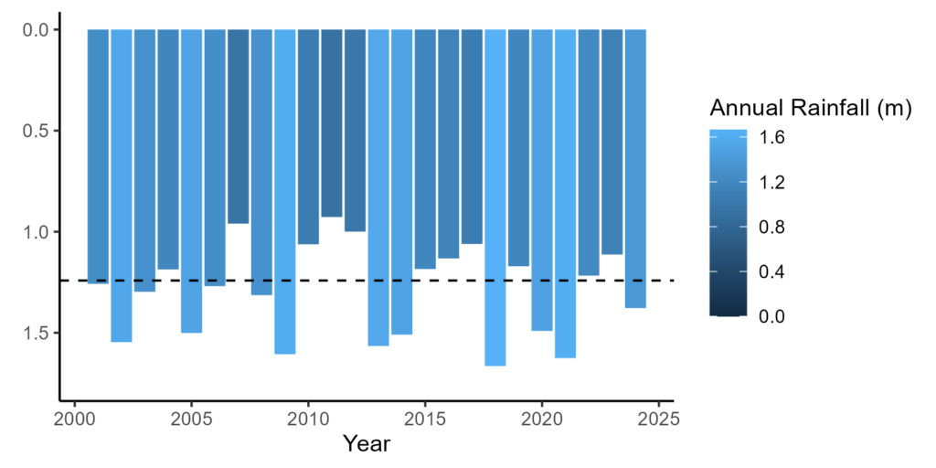
Another way to examine the normality of when rainfall occurs is through cumulative rainfall plots. In this analysis, we take the rainfall amounts from each day in a given year and cumulatively add one day’s rainfall to the following day. The final values end up making Figure 4 (above), but we can follow the path of one year’s rainfall to identify large jumps in rain (like a hurricane) or periods of flat rainfall (dry periods or droughts). Just as with the total annual rain, 2024 was a ‘normal’ year.
p1 <- ggplot(all,
             aes(x = jday,
                 y = cum_rain_m,
                 color = factor(year),
                 group = factor(year)))+
  geom_line()+
  gghighlight::gghighlight(year == 2024)+
  # ggrepel::geom_label_repel(aes(label = label),
  #                           nudge_x = 100,
  #                           label.size = 0.25,
  #                           size = 4,
  #                           hjust = 0,
  #                           show.legend = FALSE)+
  labs(x = 'Day of Year',
       y = 'Cumulative Annual Rainfall (m)')+
  scale_color_viridis_d(name = 'Year')
p1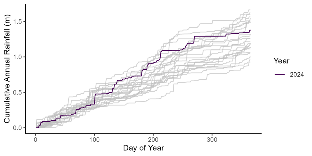
Deviation from ‘Normal’?
Finally, with the full dataset, we can calculate the average monthly rainfall to identify seasonal patterns with more data. In the graph, the mean monthly rainfall is shown in the blue line, and the 2024 monthly rainfall are the bars. This visualization allows us to clearly see the deviation from ‘normal’ conditions in 2024, particularly in July and September (wetter) and October (drier). Interesting to think about what ‘normal’ means. We use a summary statistic, like the mean monthly rainfall or average annual rainfall, to define what is the usual conditions. But the probability that an individual day or month or year will have the exact amount of rainfall as the average conditions to be ‘normal’ are effectively 0.
df_2024_month <- df_2024 %>%
  group_by(month = lubridate::month(Date,abbr = TRUE, label = TRUE)) %>%
  summarise(daily_rain = sum(`Rain mm`, na.rm = TRUE)) %>%
  filter(!is.na(month))

mean_mon_tots <- all %>%
  group_by(month = lubridate::month(date, label = TRUE, abbr = TRUE),
           year = lubridate::year(date)) %>%
  summarise(mean_yrmon_rain = 10*sum(rain_tot_cm, na.rm = TRUE)) %>%
  group_by(month) %>%
  summarise(mean_mon_rain = mean(mean_yrmon_rain, na.rm = TRUE)) %>%
  filter(!is.na(month))

ggplot(data = cbind(df_2024_month,
                    mean_mon_tots)[,c(1,2,4)],
       aes(x = month))+
  geom_bar(aes(y = daily_rain),
           stat = 'identity')+
  geom_line(aes(y = mean_mon_rain,
                group = 1,
                color = 'Mean Monthly Rainfall'),
            linewidth = 2)+
  scale_color_manual(name = element_blank(),
                     values = 'blue')+
  lims(y = c(300, 0))+
  labs(x = element_blank(),
       y = 'Rainfall (mm/month)')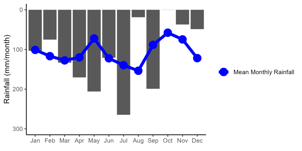
That’s a wrap from us! We’ll see you again next January with an update for 2025! Be sure to keep tabs on the drought conditions in the Apalachicola-Chattahoochee-Flint watershed here from our partners at NOAA.